Public Transportation Time Series Analysis
Tyler Young
Policy Question:
Does adding more busses to a public transportation like increase ridership in a city?
Load Data
Assigning example passenger data to a variable, and creating a control and a treatment group for analysis divided by each half of attendance throughout the year & putting this within a datframe for analysis and visualization.
Example Data from DS4PS Github.
#Passenger data

passengers <-
c(1328, 1407, 1425, 1252, 1287, 1353, 1301, 1294, 1336, 1371,
1408, 1326, 1364, 1295, 1320, 1260, 1347, 1316, 1287, 1292, 1259,
1349, 1274, 1365, 1317, 1341, 1316, 1313, 1285, 1369, 1309, 1446,
1422, 1397, 1358, 1310, 1294, 1373, 1161, 1320, 1376, 1335, 1382,
1455, 1374, 1267, 1318, 1370, 1297, 1391, 1269, 1341, 1238, 1391,
1296, 1260, 1330, 1447, 1296, 1389, 1278, 1319, 1333, 1372, 1325,
1299, 1299, 1312, 1352, 1355, 1404, 1317, 1330, 1325, 1368, 1311,
1310, 1242, 1247, 1366, 1401, 1282, 1298, 1301, 1341, 1353, 1398,
1352, 1300, 1442, 1365, 1411, 1360, 1100, 1334, 1336, 1274, 1303,
1487, 1341, 1436, 1294, 1390, 1338, 1400, 1325, 1352, 1353, 1288,
1304, 1338, 1355, 1212, 1386, 1426, 1380, 1425, 1287, 1337, 1288,
1348, 1308, 1402, 1370, 1401, 1363, 1312, 1457, 1367, 1320, 1338,
1447, 1371, 1402, 1461, 1382, 1260, 1341, 1309, 1317, 1509, 1403,
1324, 1347, 1351, 1307, 1267, 1312, 1472, 1403, 1327, 1501, 1470,
1438, 1416, 1369, 1355, 1317, 1448, 1423, 1401, 1356, 1400, 1356,
1452, 1435, 1387, 1372, 1390, 1538, 1460, 1474, 1510, 1360, 1424,
1275, 1381, 1453, 1430, 1404, 1350, 1375, 1327, 1312, 1464, 1478,
1536, 1397, 1229, 1337, 1442, 1316, 1455, 1312, 1505, 1440, 1408,
1429, 1280, 1560, 1422, 1363, 1349, 1326, 1400, 1464, 1488, 1352,
1485, 1446, 1540, 1435, 1377, 1287, 1480, 1353, 1359, 1493, 1387,
1314, 1478, 1306, 1462, 1533, 1261, 1488, 1482, 1461, 1452, 1540,
1438, 1423, 1425, 1353, 1489, 1546, 1401, 1459, 1527, 1341, 1516,
1406, 1414, 1442, 1272, 1371, 1435, 1446, 1287, 1496, 1442, 1614,
1305, 1459, 1342, 1478, 1501, 1357, 1428, 1444, 1431, 1425, 1434,
1488, 1508, 1454, 1436, 1485, 1522, 1437, 1396, 1407, 1382, 1444,
1494, 1303, 1552, 1282, 1352, 1412, 1378, 1579, 1543, 1425, 1404,
1380, 1593, 1555, 1532, 1514, 1485, 1504, 1442, 1401, 1453, 1493,
1522, 1417, 1545, 1422, 1540, 1447, 1447, 1575, 1431, 1516, 1542,
1519, 1485, 1526, 1400, 1563, 1471, 1517, 1506, 1514, 1444, 1348,
1588, 1574, 1275, 1331, 1436, 1475, 1570, 1513, 1469, 1573, 1432,
1467, 1513, 1475, 1572, 1430, 1512, 1532, 1487, 1474, 1508, 1410,
1455, 1445, 1544, 1500, 1517, 1496, 1606, 1613, 1526, 1487, 1540,
1511, 1534, 1620, 1409, 1542, 1517, 1493, 1443, 1463, 1391, 1583,
1516, 1700, 1422)


time <- 1:365  # or 1:length(passengers)

# sequence of 5 zeros followed by 5 ones:
treat <- c( rep(0,182), rep(1,183) )
# or using an ifelse statement since we know it starts in period 6
treat <- ifelse( time > 182, 1, 0 )

# sequence of 5 zeros followed by new counter
time.since <- c( rep(0,182), 1:183 )

d <- data.frame( passengers, time, treat, time.since )
Preview data then differentiating passengers between treatment and control groups into time periods.
d$passengers <- round(d$passengers,1)

d.sum <- rbind( head(d), c("...","...","...","..."),
                 d[ 181:184, ],
                 c("**START**","**TREATMENT**","---","---"),
                 d[ 185:189, ],
                 c("...","...","...","..."),
                 tail(d) )

row.names( d.sum ) <- NULL
pander( d.sum )| passengers | time | treat | time.since |
|---|---|---|---|
| 1328 | 1 | 0 | 0 |
| 1407 | 2 | 0 | 0 |
| 1425 | 3 | 0 | 0 |
| 1252 | 4 | 0 | 0 |
| 1287 | 5 | 0 | 0 |
| 1353 | 6 | 0 | 0 |
| … | … | … | … |
| 1350 | 181 | 0 | 0 |
| 1375 | 182 | 0 | 0 |
| 1327 | 183 | 1 | 1 |
| 1312 | 184 | 1 | 2 |
| START | TREATMENT | — | — |
| 1464 | 185 | 1 | 3 |
| 1478 | 186 | 1 | 4 |
| 1536 | 187 | 1 | 5 |
| 1397 | 188 | 1 | 6 |
| 1229 | 189 | 1 | 7 |
| … | … | … | … |
| 1463 | 360 | 1 | 178 |
| 1391 | 361 | 1 | 179 |
| 1583 | 362 | 1 | 180 |
| 1516 | 363 | 1 | 181 |
| 1700 | 364 | 1 | 182 |
| 1422 | 365 | 1 | 183 |
Plot passengers ridership by days with inflection point for analysis on treatment group.
plot( d$time, d$passengers,
      bty="n", pch=19, col="gray",
      ylim = c(1000, 2000), xlim=c(0,400),
      xlab = "Time (days)",
      ylab = "Ridership" )

# Line marking the interruption
abline( v=200, col="firebrick", lty=2 )
text( 195, 2000, "Start of New Bus Schedule", col="firebrick", cex=1.3, pos=4 )

# Add the regression line
ts <- lm( passengers ~ time + treat + time.since, data=d )
lines( d$time, ts$fitted.values, col="steelblue", lwd=2 )
#ts_d <- lm( passengers ~ time + treat + time.since, data=d )
#lines(d$passengers, col="steelblue", lwd=2 )
#lines( rep(1:365), col="dodgerblue4", lwd = 3 )Creating Treatment Group Y=b0+b1∗Time+b2∗Treatment+b3∗TimeSinceTreatment+e We can run the model using the lm function in R.
# Passenger model variables
# y=pass, t=days, d=treatment/schedule p=time since treatment

reg_d = lm ( passengers ~ time + treat + time.since)  # Our time series model

stargazer( reg_d,
           type = "text",
           dep.var.labels = ("Ridership"),
           column.labels = ("Model results"),
           covariate.labels = c("Time", "Treatment",
                                "Time Since Treatment"),
           omit.stat = "all",
           digits = 2 )
##
## ================================================
## Dependent variable:
## ---------------------------
## Ridership
## Model results
## ------------------------------------------------
## Time 0.46***
## (0.10)
##
## Treatment -2.37
## (14.24)
##
## Time Since Treatment 0.22
## (0.14)
##
## Constant 1,310.27***
## (10.13)
##
## ================================================
## ================================================
## Note: *p<0.1; **p<0.05; ***p<0.01Let’s interpret our coefficients: The Time coefficient indicates the ridership trend before the schedule change It’s positive and significant, indicating that ridership is increasing over time. For each day that passes, buses gain just under half a rider. The Treatment coefficient indicates the increase or decrease in ridership immediately after the schedule intervention. We can see that the immediate effect is negative indicating that ridership went down by 2.37 people. The Time Since Treatment coefficient indicates that the trend has changed after the intervention. The sustained effect is positive indicating that for each day that passes after the intervention, the bus ridership increases of 0.22 people. (These results may not be statistically significant, though we may cannot yet tell at this point) Plotting the results A useful exercise is to calculate outcomes at different points in time. For instance, we can calculate the outcome right after the intervention, which occurred at time = 182. Note that while Time = 183, Time Since Treatment is equal to 1 because it is the first day after the intervention. Y=b0+b1∗201+b2∗1+b3∗1+e We can also represent the point on a graph:
# We create a small dataset with the new values
data1 <- as.data.frame( cbind( time = 184, treat = 1, time.since = 1 ))

# We use the function predict to (1) take the
#  coefficients estimated in reg_d and
#  (2) calculate the outcome Y based on the
#  values we set in the new datset
y1 <- predict( reg_d, data1 )


# We plot our initial observations, the column Y (passengers) in our dataset
plot( passengers,
      bty="n",
      col = gray(0.5,0.5), pch=19,
      xlim = c(1, 365),
      ylim = c(1000, 2000),
      xlab = "Time (days)",
      ylab = "Ridership")

# We add a point showing the level of ridership at time = 184)
points( 184, y1, col = "dodgerblue4",
        pch = 19, bg = "dodgerblue4", cex = 2 )
text( 184, y1, labels = "t = 184", pos = 4, cex = 1 )

# Line marking the interruption
abline( v=183, col="red", lty=2 )
Now, we can calculate the outcome 30 days after the intervention. Time will be equal to 214 while Time Since Treatment will be equal to 30. Treatment is always equal to 1 since it is a dummy variable indicating pre or post intervention. Y=b0+b1∗230+b2∗1+b3∗30+e We can add the new point at t = 214 to the graph:
data2 <- as.data.frame( cbind( time = 214, treat = 1, time.since = 30 )) # New data

y2 <- predict( reg_d, data2 ) # We predict the new outcome

# We plot our initial observations, the column Y in our dataset
plot( passengers,
      bty="n",
      col = gray(0.5,0.5), pch=19,
      xlim = c(1, 365),
      ylim = c(1000, 2000),
      xlab = "Time (days)",
      ylab = "Ridership")

# We add a point showing the level of ridership at time = 184
points(184, y1, col = "dodgerblue4", pch = 19, bg = "red", cex = 2)

# We add a new point showing the level of ridership at time = 214)
points(214, y2, col = "dodgerblue4", pch = 19, bg = "red", cex = 2)

# Label for our predicted outcome
text(184, y1, labels = "t = 184", pos = 1, cex = 1)

#Label for the counterfactual
text(214, y2, labels = "t = 214", pos = 4, cex = 1, )

# Line marking the interruption
abline( v=183, col="red", lty=2 )
The Counterfactual; We can calculate the counterfactual for any point in time. The counterfactual at Time = 214 is the level of ridership at that point in time if the intervention had not occured. Note the changes in our equation: Treatment and Time Since Treatment are both equal to 0. Y=b0+b1∗230+b2∗0+b3∗0+e As before, we plot the results on a graph. Y is our predict value and C is the counterfactual
d5 <- as.data.frame(cbind( time= 214, treat = 0, time.since = 0)) # Data if the intervention does not occur

y3 <- predict(reg_d, d5) #Counterfactual

# We plot our initial observations, the column Y in our dataset
plot( passengers,
      bty="n",
      col = gray(0.5,0.5), pch=19,
      xlim = c(1, 365),
      ylim = c(1000, 2000),
      xlab = "Time (days)",
      ylab = "Ridership")

# We add a  point showing the level of ridsership at time = 214
points(214, y2, col = "dodgerblue4", pch = 19, bg = "red", cex = 2)

# We add a point indicating the counterfactual
points(214, y3, col = "darkorange2", pch = 19, cex = 2)

# Label for our predicted outcome
text(214, y2, labels = "Y at t = 230", pos = 3, cex = 1)

#Label for the counterfactual
text(214, y3, labels = "C at t = 230", pos = 1, cex = 1)

# Line marking the interruption
abline( v=183, col="red", lty=2 )
Let’s zoom in th see the minimal change
d5 <- as.data.frame(cbind( time= 214, treat = 0, time.since = 0)) # Data if the intervention does not occur

y3 <- predict(reg_d, d5) #Counterfactual

# We plot our initial observations, the column Y in our dataset
plot( passengers,
      bty="n",
      col = gray(0.5,0.5), pch=19,
      xlim = c(184, 230),
      ylim = c(1400, 1430),
      xlab = "Time (days)",
      ylab = "Ridership")

# We add a  point showing the level of ridsership at time = 214
points(214, y2, col = "dodgerblue4", pch = 19, bg = "red", cex = 2)

# We add a point indicating the counterfactual
points(214, y3, col = "darkorange2", pch = 19, cex = 2)

# Label for our predicted outcome
text(214, y2, labels = "Y at t = 230", pos = 1, cex = 1)

#Label for the counterfactual
text(214, y3, labels = "C at t = 230", pos = 1, cex = 1)

# Line marking the interruption
abline( v=183, col="red", lty=2 )

text( 200, 1422, "Statistically Insignificant Change", col="firebrick", cex=1.0, pos=4 )
This changes only slightly by choosing different days to compare.
d6 <- as.data.frame(cbind( time = 320, treat = 1, time.since =183))
d7 <- as.data.frame(cbind( time = 320, treat = 0, time.since = 0))

y4 <- predict(reg_d, d6)
y5 <- predict(reg_d, d7)

# We plot our initial observations, the column Y in our dataset
plot( passengers,
      bty="n",
      col = gray(0.5,0.5), pch=19,
      xlim = c(1, 365),
      ylim = c(1000, 2000),
      xlab = "Time (days)",
      ylab = "Ridership")

# ridership at time = 214
points(214, y2, col = "dodgerblue4", pch = 19, bg = "red", cex = .6)

# Counterfactual at time = 214
points(214, y3, col = "darkorange2", pch = 19, cex = .6)

# ridership at time = 320
points(320, y4, col = "dodgerblue4", pch = 19, cex = .6)

# Counterfactual at time = 320
points(320, y5, col = "darkorange2", pch = 19, cex = .6)

# Adding labels
text(320, y4, labels = "Y at t=320", pos = 4, cex = .9)
text(320, y5, labels = "C at t=320", pos = 4, cex = .9)
text(230, y2, labels = "Y at at=214", pos = 1, cex = 1)
text(230, y3, labels = "C at t=214", pos = 4, cex = 1)

# Line marking the interruption
abline( v=183, col="red", lty=2 )
Again, they are very close together, at 30 days post policy, however they are further separated at 183 days after thew policy, and we can now plot the predicted outcomes of the policy change.
pred1 <- predict(reg_d, d)
# To estimate all predicted values of Y, we just use our dataset

datanew <- as.data.frame(cbind(time = rep(1 : 365), treat = rep(0), passengers = rep(0)))
# Create a new dataset where Treatment and Time Since Treatment are equal to 0 as the intervention did not occur.

pred2 <- predict(reg_d, datanew)
# Predict the counterfactuals

plot( passengers,
      bty="n",
      col = gray(0.5,0.5), pch=19,
      xlim = c(1, 365),
      ylim = c(1000, 2000),
      xlab = "Time (days)",
      ylab = "Ridership")

lines( rep(1:182), pred1[1:182], col="dodgerblue4", lwd = 3 )
lines( rep(184:365), pred1[184:365], col="dodgerblue4", lwd = 3 )
lines( rep(183:365), pred2[183:365], col="darkorange2", lwd = 3, lty = 5 )

text(0, 1200, labels = "Predicted values", pos = 4, cex = 1, col = "dodgerblue3")
text(300, 1400, labels = "Counterfactual", pos = 4, cex = 1, col = "darkorange2")

# Line marking the interruption
abline( v=183, col="darkorange2", lty=2 )
A Closer look into the predicted change.
pred1 <- predict(reg_d, d)
# To estimate all predicted values of Y, we just use our dataset

datanew <- as.data.frame(cbind(time = rep(1 : 365), treat = rep(0), passengers = rep(0)))
# Create a new dataset where Treatment and Time Since Treatment are equal to 0 as the intervention did not occur.

pred2 <- predict(reg_d, datanew)
# Predict the counterfactuals

plot( passengers,
      bty="n",
      col = gray(0.5,0.5), pch=19,
      xlim = c(180, 365),
      ylim = c(1350, 1520),
      xlab = "Time (days)",
      ylab = "Ridership")

lines( rep(1:182), pred1[1:182], col="dodgerblue4", lwd = 3 )
lines( rep(184:365), pred1[184:365], col="dodgerblue4", lwd = 1.5 )
lines( rep(183:365), pred2[183:365], col="darkorange2", lwd = 1.5, lty = 5 )

text(0, 1200, labels = "Predicted values", pos = 4, cex = 1, col = "dodgerblue3")
text(300, 1400, labels = "Counterfactual", pos = 4, cex = 1, col = "darkorange2")

# Line marking the interruption
abline( v=183, col="darkorange2", lty=2 )
As we can see, there is a marginal increase in ridership however we do not know the difference.
Delayed Effects in Time Series
Note that the coefficients obtained from the previous equations do not tell us if the difference between each point (the predicted outcomes) and its counterfactual is statistically significant. They only tell you if there is an immediate change after the intervention and the slope has changed after the intervention. There is no statistical test to look at whether there is a statistically significant difference between a predicted outcome and its counterfactual. This has important implications. It could be that effect of the intervention varies over time.
reg_d2 = lm(passengers ~ time + treat + time.since, data = d)

stargazer( reg_d2,
           type = "text",
           dep.var.labels = ("Ridership"),
           column.labels = ("Model results"),
           covariate.labels = c("Time", "Treatment", "Time Since Treatment"),
           omit.stat = "all",
           digits = 2 )
##
## ================================================
## Dependent variable:
## ---------------------------
## Ridership
## Model results
## ------------------------------------------------
## Time 0.46***
## (0.10)
##
## Treatment -2.37
## (14.24)
##
## Time Since Treatment 0.22
## (0.14)
##
## Constant 1,310.27***
## (10.13)
##
## ================================================
## ================================================
## Note: *p<0.1; **p<0.05; ***p<0.01Measuring at day 300
pred1 <- predict(reg_d, d)
# To estimate all predicted values of Y, we just use our dataset

datanew <- as.data.frame(cbind(time = rep(1 : 365), treat = rep(0), passengers = rep(0)))
# Create a new dataset where Treatment and Time Since Treatment are equal to 0 as the intervention did not occur.

pred2 <- predict(reg_d, datanew)
# Predict the counterfactuals

plot( passengers,
      bty="n",
      col = gray(0.5,0.5), pch=19,
      xlim = c(1, 365),
      ylim = c(1000, 2000),
      xlab = "Time (days)",
      ylab = "Ridership")

lines( rep(1:182), pred1[1:182], col="dodgerblue4", lwd = 3 )
lines( rep(184:365), pred1[184:365], col="dodgerblue4", lwd = 3 )
lines( rep(183:365), pred2[183:365], col="darkorange2", lwd = 3, lty = 5 )

text(0, 1200, labels = "Predicted values", pos = 4, cex = 1, col = "dodgerblue3")
text(300, 1400, labels = "Counterfactual", pos = 4, cex = 1, col = "darkorange2")

# Line marking the interruption
abline( v=183, col="darkorange2", lty=2 )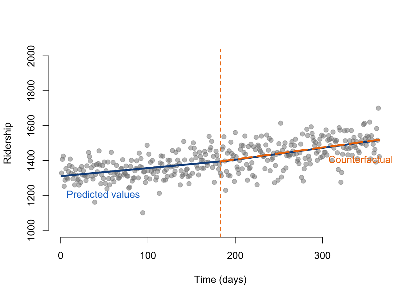
pred1 <- predict(reg_d, d)
# To estimate all predicted values of Y, we just use our dataset

datanew <- as.data.frame(cbind(time = rep(1 : 365), treat = rep(0), passengers = rep(0)))
# Create a new dataset where Treatment and Time Since Treatment are equal to 0 as the intervention did not occur.

pred2 <- predict(reg_d, datanew)
# Predict the counterfactuals

plot( passengers,
      bty="n",
      col = gray(0.5,0.5), pch=19,
      xlim = c(180, 365),
      ylim = c(1350, 1520),
      xlab = "Time (days)",
      ylab = "Ridership")

lines( rep(1:182), pred1[1:182], col="dodgerblue4", lwd = 1.5 )
lines( rep(184:365), pred1[184:365], col="dodgerblue4", lwd = 1.5 )
lines( rep(183:365), pred2[183:365], col="darkorange2", lwd = 1.5, lty = 5 )

text(0, 1200, labels = "Predicted values", pos = 4, cex = 1, col = "dodgerblue3")
text(300, 1400, labels = "Counterfactual", pos = 4, cex = 1, col = "darkorange2")

# Line marking the interruption
#abline( v=300, col="forestgreen", lty=2 )
abline( v=183, col="darkorange2", lty=2 )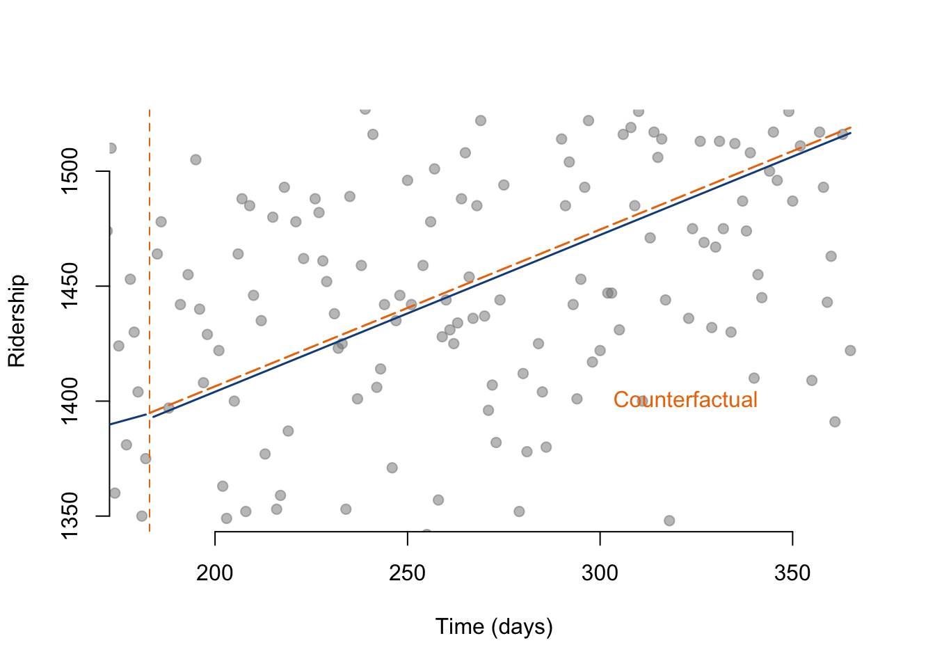
Brief analysis:
-The intercept is the constant slope of the line before the change in bus policy. -The time coefficient represents which day of the year it is. -The coefficient that represents the immediate effect of the policy would be within the time since treatment, specifically the first day after the implementation, so the 184th day of the year. -The sustained effect of the policy can be summarized as the slope of ridership over days 184-365 during the time since treatment -The policy has slightly decreased ridership in the second half of the year, we can see that the outcome was that ridership was down by just over 2 passengers, however the results were not statistically significant. -The overall trend of the policy appears to have increased ridership slightly over the time period by less than a single passenger per day, however this is not a statistically significant result. -These results can be explained by the behavior of the riders, which could have remained the same, the same number of people are taking the bus, though as the increased schedule was implemented, many of them could have simply gotten to their destinations faster due to the increased schedule.
Predicted caounterfactual of ridership compared to control
pred1 <- predict(reg_d, d)
# To estimate all predicted values of Y, we just use our dataset

datanew <- as.data.frame(cbind(time = rep(1 : 365), treat = rep(0), passengers = rep(0)))
# Create a new dataset where Treatment and Time Since Treatment are equal to 0 as the intervention did not occur.

pred2 <- predict(reg_d, datanew)
# Predict the counterfactuals

plot( passengers,
      bty="n",
      col = gray(0.5,0.5), pch=19,
      xlim = c(1, 365),
      ylim = c(1000, 2000),
      xlab = "Time (days)",
      ylab = "Ridership")

lines( rep(1:182), pred1[1:182], col="dodgerblue4", lwd = 3 )
lines( rep(184:365), pred1[184:365], col="dodgerblue4", lwd = 3 )
lines( rep(183:365), pred2[183:365], col="darkorange2", lwd = 3, lty = 5 )

text(0, 1200, labels = "Predicted values", pos = 4, cex = 1, col = "dodgerblue3")
text(300, 1400, labels = "Counterfactual", pos = 4, cex = 1, col = "darkorange2")
text(200, 1800, labels = "100 Days after Policy", pos = 4, cex = 1, col = "forestgreen")
# Line marking the interruption
abline( v=183, col="darkorange2", lty=2 )
abline( v=284, col="forestgreen", lty=2 )
d7<- as.data.frame(cbind( time= 284, treat = 0, time.since = 0)) # Data if the intervention does not occur

y7 <- predict(reg_d, d7) #Counterfactual

# We plot our initial observations, the column Y in our dataset
plot( passengers,
      bty="n",
      col = gray(0.5,0.5), pch=19,
      xlim = c(1, 365),
      ylim = c(1350, 1500),
      xlab = "Time (days)",
      ylab = "Ridership")

# We add a  point showing the level of ridsership at time = 214
points(284, y2, col = "dodgerblue4", pch = 19, bg = "red", cex = 1)

# We add a point indicating the counterfactual
points(284, y3, col = "darkorange2", pch = 19, cex = 1)

# Label for our predicted outcome
text(284, y2, labels = "Y at t = 230", pos = 3, cex = 1)

#Label for the counterfactual
text(284, y3, labels = "C at t = 230", pos = 1, cex = 1)

# Line marking the interruption
abline( v=183, col="red", lty=2 )
pred1 <- predict(reg_d, d)
# To estimate all predicted values of Y, we just use our dataset

datanew <- as.data.frame(cbind(time = rep(1 : 365), treat = rep(0), passengers = rep(0)))
# Create a new dataset where Treatment and Time Since Treatment are equal to 0 as the intervention did not occur.

pred2 <- predict(reg_d, datanew)
# Predict the counterfactuals

plot( passengers,
      bty="n",
      col = gray(0.5,0.5), pch=19,
      xlim = c(1, 365),
      ylim = c(1000, 2000),
      xlab = "Time (days)",
      ylab = "Ridership")

lines( rep(1:182), pred1[1:182], col="dodgerblue4", lwd = 3 )
lines( rep(184:365), pred1[184:365], col="dodgerblue4", lwd = 3 )
lines( rep(183:365), pred2[183:365], col="darkorange2", lwd = 3, lty = 5 )

text(0, 1200, labels = "Predicted values", pos = 4, cex = 1, col = "dodgerblue3")
text(300, 1400, labels = "Counterfactual", pos = 4, cex = 1, col = "darkorange2")
text(200, 1800, labels = "150 Days after Policy", pos = 4, cex = 1, col = "forestgreen")
# Line marking the interruption
abline( v=183, col="darkorange2", lty=2 )
abline( v=334, col="forestgreen", lty=2 )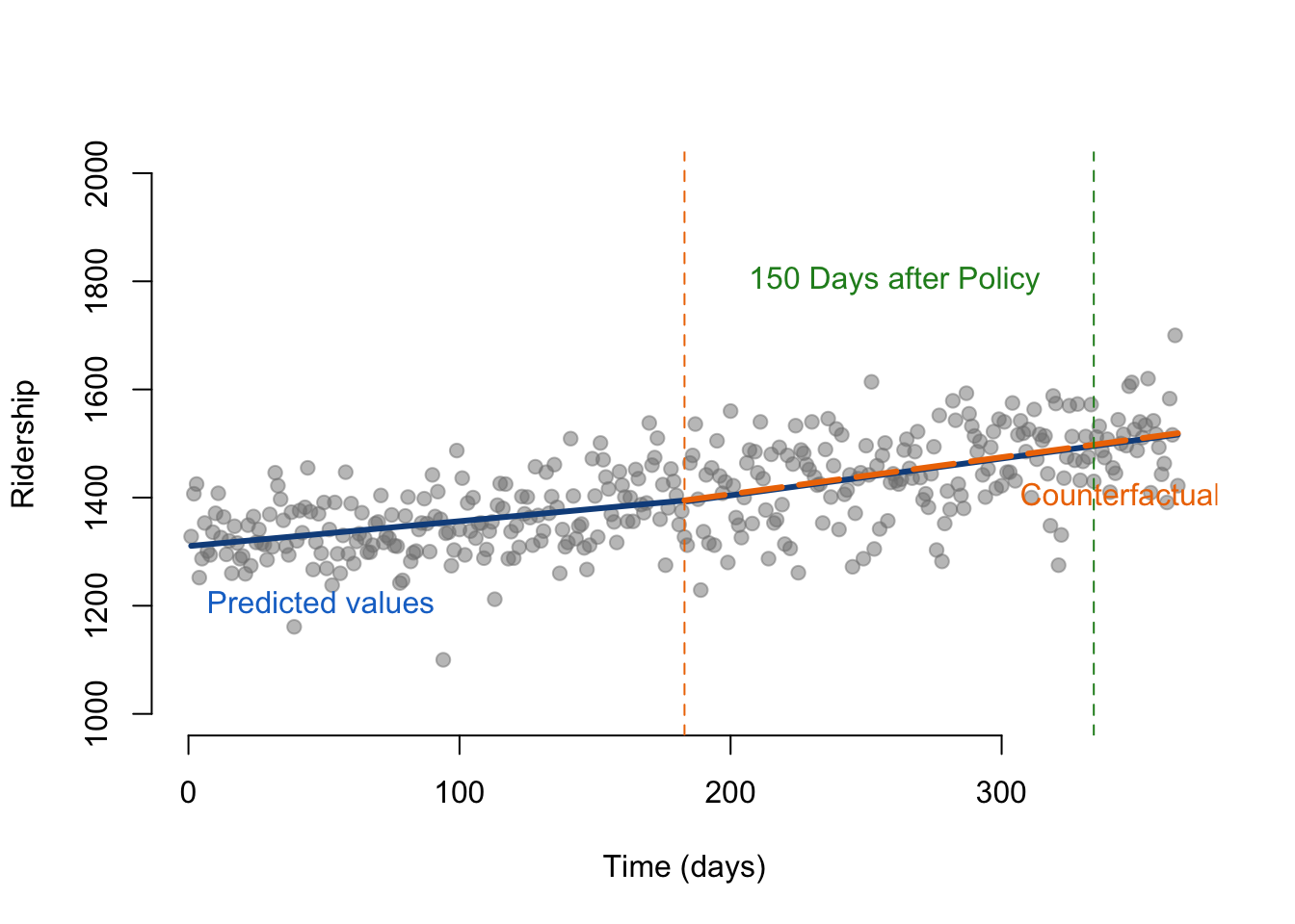
d7<- as.data.frame(cbind( time= 334, treat = 0, time.since = 0)) # Data if the intervention does not occur

y7 <- predict(reg_d, d7) #Counterfactual

# We plot our initial observations, the column Y in our dataset
plot( passengers,
      bty="n",
      col = gray(0.5,0.5), pch=19,
      xlim = c(1, 365),
      ylim = c(1350, 1500),
      xlab = "Time (days)",
      ylab = "Ridership")

# We add a  point showing the level of ridsership at time = 214
points(334, y2, col = "dodgerblue4", pch = 19, bg = "red", cex = 1)

# We add a point indicating the counterfactual
points(334, y3, col = "darkorange2", pch = 19, cex = 1)

# Label for our predicted outcome
text(334, y2, labels = "Y at t = 230", pos = 3, cex = 1)

#Label for the counterfactual
text(334, y3, labels = "C at t = 230", pos = 1, cex = 1)

# Line marking the interruption
abline( v=183, col="red", lty=2 )
Brief analysis: -The predicted number of passengers 100 days post policy is 1425 passengers -The counterfactual is the estimation of the number of passengers that would have ridden the bus should the policy not have been implemented -1475 passengers are riding 150 days post treatment -The two counterfactuals are not the same, and cannot be concluded as predictive because ridership is gradually increasing over time, regardless of the treatment policy